Adding Combustion — When the Bang Matters

Series: ← The Slider-Crank, Three Ways · ← Multi-Cylinder I4 · ← Boxer-4 · ← Rocking Couples · ← Non-boxer Flat-4 · ← Summary · ← V-Engines · Combustion · Balance Shafts → · Engine Mounts → · Active Damping → · Chassis Response → · Engine Mounts →

Reference: Field Guide · Concepts Primer · Physics · Computational Machinery · Dimensional Reduction

Every chapter so far analysed the inertial signature of a multi-cylinder engine: the reciprocating masses alone, dragged around at constant speed with no spark. That is the “motoring” spectrum — what you would feel on a dyno pulling a dead engine around.

Real engines also burn fuel. The gas pressure pulse on each piston during its power stroke is a separate forcing function that lives on a different cycle (720°, not 360°), fires at a different frequency ( $N_\text{cyl}/2$ × crank, not crank), and has its own harmonic content. This chapter adds that forcing function to the same phasor framework, without replacing any of the infrastructure from the earlier chapters.

The script: combustion_analysis.py. Presets: I4, Boxer-4, Straight-6, V8 flat-plane, V8 cross-plane — each with a realistic firing order attached.

1. Why combustion is a different beast from inertia

Mechanically, combustion pressure acts along the same axis as piston motion — so the bank-angle projection from the V-engines chapter carries over verbatim. The combustion force on the bearing from cylinder $i$ is still

$F_i(t) = F_{\text{pulse},i}(t) \cdot (\cos\beta_i,\ \sin\beta_i)$

but with two new complications:

Four-stroke period is 720°, not 360°. Each cylinder fires once every two crank revolutions, so the forcing function has period $2T_\text{crank}$ . Its harmonics therefore live at half-integer multiples of crank frequency: ½×, 1×, 1½×, 2×, … — twice as dense as the inertial harmonics.
Firing order is a new input. The piston is at TDC twice per 720° cycle (end of compression, end of exhaust), but fires at only one of them. The inertial framework can’t distinguish the two TDCs because both give the same acceleration. Combustion can, so the preset now needs a fourth per-cylinder list firing_deg: the 720° crank angle at which each cylinder fires. It must equal phases_deg[i] or phases_deg[i] + 360° (modulo 720°).

Everything else — the 2D phasor sums, the moment sums, the preset format — stays the same.

2. The parameterised combustion pulse

The real pressure trace $P(\theta)$ of an engine cylinder is a complicated thing: fast rise from spark, peak a few degrees after TDC, exponential blow-down through the expansion stroke, then roughly flat during exhaust and intake. For a first-cut vibration analysis we do not need that fidelity — we need something that fires sharply near TDC, has a realistic spectrum, and is easy to parameterise.

The default pulse in this chapter is a half-sine over a duty window:

                       |---  duty · 720°  ---|
         F_peak   ·····◦                   
                       ·         ·
                     ·             ·
                    ·               ·
                    · · · · · · · · · · · · · · · · · · ·
         0   ────·──────────────────·───────────────────────
               TDC                  end of                    (next cycle)
           (power stroke start)    power stroke
         0°         duty·720°                     720°

With two knobs:

F_peak — peak gas force on the piston in Newtons. Default 10 kN (typical for a 100 mm bore at moderate load, BMEP ~ 10 bar, peak cylinder pressure ~ 50 bar).
duty — active fraction of the 720° cycle. Default 0.25 (= 180 crank degrees of power stroke).

This is enough to reproduce the qualitative balance-of-harmonics behaviour across different engine configurations. For better realism there are two well-known upgrades:

Measured P–θ trace — tabulated pressure as a function of crank angle, plugged in directly.
Wiebe heat-release model — a physics-based heat-release fraction

$x_b(\theta) = 1 - \exp\!\left(-a \cdot \left(\frac{\theta - \theta_0}{\Delta\theta}\right)^{m+1}\right)$

with typical Wiebe constants $a \approx 5$ , $m \approx 2$ , converted to pressure through a cycle analysis.

Both are drop-in replacements for build_pressure_pulse(). The phasor framework doesn’t care which of these produced F_pulse[k] — it just consumes per-harmonic amplitudes. See FAQ §5 for the full story.

3. The phasor framework reused

For the inertial chapters we had, at crank harmonic $n$ :

$\hat{F}_\text{total}[n] = \hat{F}_\text{single}[n] \cdot \sum_i \exp(j \cdot n \cdot \phi_i) \qquad \text{(1D, inline)}$

$\hat{F}_\text{total}^{x,y}[n] = \hat{F}_\text{single}[n] \cdot \sum_i \cos\ \text{or}\ \sin(\beta_i) \cdot \exp(j \cdot n \cdot \phi_i) \qquad \text{(V-engine)}$

For combustion, the indexing is identical — we just re-interpret $\phi_i$ as the firing angle in the 720° cycle (mapped to $[0, 2\pi)$ ), and $n$ as the harmonic of the 720° cycle:

$\hat{F}_\text{total}^{x,y}[k] = \hat{F}_\text{pulse}[k] \cdot \sum_i \cos\ \text{or}\ \sin(\beta_i) \cdot \exp(j \cdot k \cdot \psi_i)$

where $\psi_i = \text{firing\_deg}_i \cdot \pi / 360$ and $k$ indexes harmonics of the 720° cycle (so $k = 1$ is ½× crank, $k = 2$ is 1× crank, …, $k = N_\text{cyl}$ is firing frequency).

Moments sum the same way, weighted by $x_i$ . Under the hood it’s the same phasor_sum_2d() and phasor_moment_sum_2d() functions from _common.py — zero new math, zero new infrastructure.

4. Numerical results — the headline table

Running python combustion_analysis.py at F_peak = 10 kN, duty = 0.25, cylinder half-spacing a = 100 mm:

Pulse harmonics (single-cylinder reference, N):
  k=0 (   0x crank):  1591.54     (DC component = mean thrust)
  k=1 ( 0.5x crank):  3001.04     (fundamental of 720° cycle)
  k=2 (   1x crank):  2500.00
  k=3 ( 1.5x crank):  1800.65
  k=4 (   2x crank):  1061.05
  k=5 ( 2.5x crank):   428.74

| Config | DC |F| | ½× |F| | 1× |F| | 1½× |F| | 2× |F| | 2½× |F| | Firing-freq |F| | |---|---:|---:|---:|---:|---:|---:|---:| | I4 (1-3-4-2) | 6366 N | 0 | 0 | 0 | 4244 N | 0 | 4244 N (= 2×) | | Boxer-4 (1-3-2-4) | 0 | 8488 N | 0 | 5093 N | 0 | 1213 N | 0 | | Straight-6 (1-5-3-6-2-4) | 9549 N | 0 | 0 | 0 | 0 | 0 | 0 (see §6 Q3) | | V8 flat-plane | 9003 N (y) | 0 | 0 | 0 | 6002 N (x) | 0 | 1201 N (y) | | V8 cross-plane | 9003 N (y) | 4594 N (x) | 0 | 6654 N (x) | 0 | 1584 N (x) | 1201 N (y) |

Moments (same configs, headline rows only):

| Config | ½× |M| | 1× |M| | 1½× |M| | |---|---:|---:|---:| | I4 | 1898 N·m (pitch) | 0 | 1139 N·m (pitch) | | Boxer-4 | 849 N·m (pitch) | 0 | 509 N·m (pitch) | | Straight-6 | 1040 N·m (pitch) | 0 | 1621 N·m (pitch) | | V8 flat-plane | 1340 N·m | 0 | 807 N·m | | V8 cross-plane | 1131 N·m | 1000 N·m | 432 N·m |

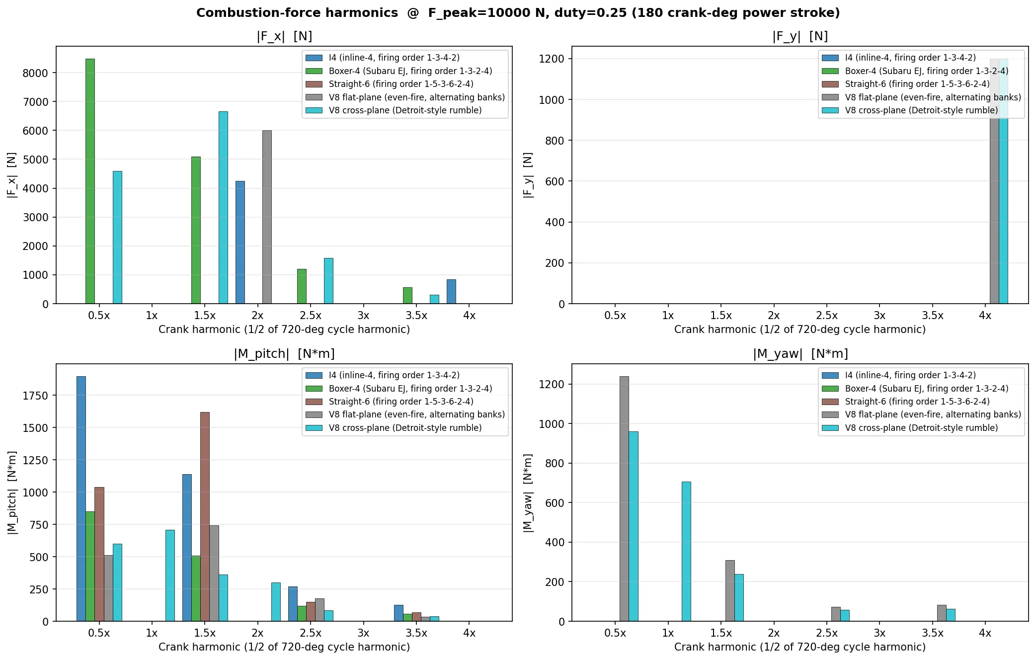
Combustion comparison across engines

5. Reading the results

I4 firing-frequency beat at 2× crank = 4.24 kN

The I4 is the textbook case: four cylinders fire 180° apart in the 720° cycle, so all four firings arrive at the bearing with the same phase at harmonic $k = 4$ . Result is a 4244 N peak force at 2× crank — the same direction (inline-x) as the inertial 2× secondary shake, and 260× bigger than the inertial 2× (~16.4 N). Below idle the inertial part dominates; above idle the combustion firing beat dominates. Both live at the same frequency. Balance shafts cancel the inertial 2× but do nothing for the combustion 2× — that is why an I4 is always noisier than a 6-cylinder at 2× crank even with perfect balance hardware.

Boxer-4 cancels at firing frequency (good) but not at ½×/1½× (surprise)

The boxer’s opposed banks with alternating firings $[0°, 180°, 360°, 540°]$ give complete cancellation at every integer-crank harmonic (1×, 2×, 3×, …) including the firing frequency of 2×. But at half-integer-crank harmonics (½×, 1½×, 2½×) the boxer has huge combustion forces — 8.5 kN at ½×, 5.1 kN at 1½×. This is the boxer-specific “low-frequency rumble” that owners of Subaru EJ engines know as the distinctive sound signature. The 720°-cycle asymmetry (cyl 1 fires once at 0°, cyl 3 once at 180°, then cyl 2 once at 360° and cyl 4 at 540°) puts energy at half-order harmonics that inertial analysis never sees, because inertia only cares about 360°-periodic effects.

V8 flat-plane vs cross-plane — back-to-back contrast

Both V8s have the same F_peak, same duty, same bank geometry, same positions, same firing frequency. The difference is which cylinder fires at each 90° firing slot.

Flat-plane has perfectly alternating R-L firing at every 90°. This gives zero force at every half-integer harmonic (½×, 1½×, 2½×, 3½×) — the engine is smooth below firing frequency — but puts a massive 6 kN at 2× crank and the firing frequency 1.2 kN at 4× crank (world-y direction). The NVH signature is a high-pitched “buzz” at 2× and 4× crank with nothing in between. Classic Ferrari V8 wail.
Cross-plane has R-L-R-R-L-R-L-L firing pattern (two same-bank fires in a row twice per cycle). This breaks the half-integer cancellation and puts 4.6 kN at ½×, 6.7 kN at 1½×, and 1.6 kN at 2½× crank — a dense mix of low-frequency harmonics that flat-plane doesn’t have. Detroit calls this “rumble”; NVH engineers call it “un-even firing interval” vibration. The reason American V8s sound the way they do is entirely captured in this one firing-order difference.

V8 flat vs cross combustion harmonics

Straight-6 at firing frequency — pulse-shape caveat

Geometrically the I6 adds constructively at firing frequency ( $k = 6$ = 3× crank): all six firings at 120° spacing are a perfect $\exp(j \cdot 2\pi \cdot m)$ pattern for the full cycle, and the bank projection gives $\sum \cos(0) \cdot 1 = 6$ . But the numerical result is zero because the duty = 0.25 half-sine pulse has a spectral zero at k = 6 (half-sine of width W has nulls at frequencies of $2k/W - 1$ for odd k; here that lands on k = 6). A real engine pulse has no such perfect null, so a real I6 does produce a 3× crank firing-frequency peak. This is a pulse-shape artefact, not an engine-balance result.

The right reading of the result is: the I6’s geometric cancellation is real at every other harmonic, and its 3× firing-frequency peak is determined by whatever spectral content the pulse shape has at k = 6. Use a Wiebe or measured trace and you’ll see the peak.

6. The big picture — inertial vs combustion, together

Putting it all in one view for a ~10 RPM 100 mm-bore 2 m-stroke (the default test engine), per cylinder:

Source	1× crank	2× crank
Inertial (from summary chapter)	9.87 N	4.11 N
Combustion (this chapter, F_peak = 10 kN)	2500 N	1061 N

At these operating conditions combustion dominates by 2–3 orders of magnitude. This is why serious NVH analysis at typical engine operating points focuses on combustion harmonics, not inertial. Inertial analysis matters at very high RPM (inertial scales as $\omega^2$ , so at 6000 RPM the 9.87 N scales up to ~36 kN per cylinder) and for balance-hardware design, where inertial forces are the thing balance shafts actually cancel.

Both live in the same phasor framework, summed the same way, reported in the same units. You can read off from a single table whether a given harmonic is inertia-dominated, combustion-dominated, or a mix.

7. FAQ

Q1. Why is the combustion force 250× bigger than the inertial force?

Because F_peak = 10 kN is a realistic gas-pressure load, while the inertial force at 10 RPM is basically ambient — the slider moves slowly, $m \cdot \omega^2 \cdot R \approx 5\ \text{kg} \cdot (\pi/3)^2 \cdot 1\ \text{m} \approx 5.5\ \text{N}$ . Scale $\omega$ up to 6000 RPM (a factor of 600× in rpm, so 360000× in $\omega^2$ ) and the inertial force becomes comparable to combustion. At idle speeds combustion dominates; at race RPMs inertia catches up and then takes over. The framework is linear in both, so you can compute at any operating point and read the ratios.

Q2. Why does the cross-plane V8 have moments at integer crank harmonics (1× crank = 1 kN·m) while flat-plane doesn’t?

Same reason as the inertial version: flat-plane’s symmetric firing pattern (perfectly alternating R-L with mirror-image x-positions) cancels odd-crank moments exactly, while cross-plane’s un-even bank pattern doesn’t. The cross-plane’s famous 1× crank rocking couple shows up in both inertial AND combustion analysis, because both forcing functions are along the same bore-axis direction and both inherit the geometric asymmetry. Inertial 1× rocking (from V-engines chapter) = 2.79 N·m; combustion 1× rocking = 1000 N·m. Both present, combustion dominating by 360×.

Q3. Why does my straight-6 show zero at firing frequency — that can’t be right?

It’s a pulse-shape artefact, not an engine property. The duty = 0.25 half-sine pulse has a Fourier spectral zero at $k = 6$ (3× crank). With a smoother, more realistic pulse — say the Wiebe heat-release model described in Q5 below — the I6’s firing-frequency peak is fully present (3× crank force equal to 6 × $F_\text{pulse}[6]$ , and $F_\text{pulse}[6]$ is non-zero for any real pulse). Try running the script with duty = 0.4 or any other value; the zero moves and the I6 firing-freq peak appears.

Takeaway: the phasor coefficient (which tells you the engine’s balance property) is independent of pulse shape. The absolute force depends on pulse shape. Engineering analysis of a real engine needs both.

Q4. How do I analyse my own engine in this framework?

Four per-cylinder lists and you are done:

my_engine = dict(
    phases_deg       = [...],   # inertial phases, 0-360 deg
    bank_angles_deg  = [...],   # bore directions, 0-360 deg from world +x
    positions        = [...],   # x along crankshaft, metres
    firing_deg       = [...],   # firing angles in 720-deg cycle
)

Then analyse(my_engine, F_pulse, n_harmonics=8) gives you every harmonic. All the existing presets in _build_presets() are worked-out examples to copy.

Q5. How would I replace the half-sine with a more realistic pulse?

Drop-in replacement for build_pressure_pulse(). Two common upgrades:

Measured P–θ trace. Instrument a real engine on a dyno with a pressure transducer. Tabulate $P(\theta)$ over a full 720° cycle. Multiply by piston area $A_p$ to get force $F(\theta) = P(\theta) \cdot A_p$ . That array of samples IS your build_pressure_pulse() output. No other changes — the FFT in pulse_harmonics() consumes it without caring about shape.

Wiebe heat-release model. Physics-based: burned-fuel fraction

$x_b(\theta) = 1 - \exp\!\left(-a \cdot \left(\frac{\theta - \theta_0}{\Delta\theta}\right)^{m+1}\right)$

with typical $a \approx 5$ , $m \approx 2$ , $\Delta\theta \approx 60°$ combustion duration, $\theta_0 \approx \text{TDC} - 15°$ spark advance. Convert $x_b$ to heat release $dQ/d\theta$ , integrate the energy equation for cylinder pressure with compression/expansion isentropic bounds, get $P(\theta)$ , multiply by piston area. That is what modern GT- Power and Ricardo-WAVE solvers do. Again: all of this slots in behind build_pressure_pulse() with no change elsewhere in the framework.

For this chapter we stayed with the parameterised half-sine because it is (a) parameterisable by two numbers a non-combustion-specialist can reason about, (b) analytical enough that you can predict the spectral zeros by hand (see Q3), and (c) sufficient to reproduce the qualitative harmonic-content differences between engine types. Upgrade to Wiebe or measured P–θ when you need absolute numbers to compare against bench-test data.

Q6. What about firing-order sensitivity — how much does picking a “good” firing order matter?

A lot. Try editing the firing_deg list in the I4 preset from [0, 540, 180, 360] (order 1-3-4-2) to [0, 180, 360, 540] (order 1-2-3-4, a hypothetical “adjacent firings”). The script will re-run and show how the half-integer harmonics change (while the 2× firing- frequency peak stays the same, since it’s always $4 \cdot F_\text{pulse}[4]$ for any valid four-stroke I4 firing order). In general, the firing order is a design knob that trades off low-frequency rumble for individual-cylinder crankshaft torsional loading — real engine firing orders are chosen to balance both. This framework lets you explore that trade numerically without running a thermodynamic code.

8. What’s next

Thermodynamic pulse — replace the parameterised half-sine with a Wiebe-derived $P(\theta)$ . Script would be combustion_analysis_wiebe.py with the same preset format and harmonic output. Physical realism up; complexity up slightly; phasor framework unchanged.
Firing-order optimisation — inverse-design like the V-engine FAQ Q4: given a target low-frequency signature, solve for the firing order that minimises it. scipy.optimize over the choice of firing-pin assignment (discrete, so a small combinatorial search).
Torsional vibration — so far every harmonic we’ve computed is a lateral bearing force on the crankshaft. Combustion also excites torsional modes of the crankshaft as a flexible beam, leading to crank resonances at specific RPMs. That adds a transfer-function layer between the phasor-sum forcing and the crankshaft tip-end angle — an extension into structural dynamics rather than rigid-body.
Engine-mount transmissibility — take this (F, M) spectrum and propagate it through engine-mount stiffness and damping to the chassis. That’s where the driver actually feels it.

Files and scripts referenced

combustion_analysis.py — this chapter’s script. Produces the table in §4 and the PNG.
_common.py — the same helpers phasor_sum_2d() / phasor_moment_sum_2d() introduced for V-engines serve combustion verbatim. No new helpers.
The seven earlier chapters in the series are all linked in the navigation bar at the top of this page.