Active Mass Damping — Closing the Loop on Vibration

Series: ← The Slider-Crank, Three Ways · ← Multi-Cylinder I4 · ← Boxer-4 · ← Rocking Couples · ← Non-boxer Flat-4 · ← Summary · ← V-Engines · ← Combustion · ← Balance Shafts · ← Engine Mounts · Active Mass Damping · Chassis Response →

Reference: Field Guide · Concepts Primer · Physics · Computational Machinery · Dimensional Reduction

The Balance Shafts chapter ended with a clean result: a Lanchester pair, mechanically tuned for a single harmonic at a single operating point, brings that harmonic to zero — but only at that operating point, and only for the inertial source whose $(R/L)^2 \cdot \omega^2$ scaling matches the shaft’s own $(n\cdot\omega)^2$ scaling. Combustion harmonics (which depend on load), manufacturing imbalance (which is per-engine), cylinder deactivation (which changes the firing pattern), all leave residual vibration that no fixed mechanical balancer can handle.

The fix is to close the loop: measure the residual, compute a cancellation phasor in real time, drive an actuator. This chapter implements the simplest narrowband adaptive controller — LMS — and shows that it (a) converges to a 99.995 % cancellation in a few hundred milliseconds, (b) tracks throttle and RPM steps cleanly, and (c) goes catastrophically unstable above a critical actuator delay.

The script: active_mass_damping.py.

1. From open loop to closed loop

A passive balance shaft is open loop: design a phasor, build it into the engine, hope reality matches the design assumptions. That’s fine for the dominant inertial harmonic, which scales predictably with $\omega^2$ . It is not fine for:

Source	Why a fixed phasor fails
Combustion harmonic ripple	scales with load (BMEP), not just $\omega$
Manufacturing imbalance	each engine is slightly different
Cylinder deactivation	firing pattern changes shape entirely
Wear over engine life	mass distribution drifts
Aftermarket modifications	compression, cams, fuel — alters source

An active damper has a sensor (measuring residual block acceleration, mount-side force, or microphone pressure), a controller (computes the cancellation phasor), and an actuator (an electric or solenoid-driven force generator). The controller adapts the phasor in real time so the residual stays at zero regardless of what the engine is doing.

   F_engine(t) ──┐                            ┌─→ residual e(t)
                 ▽                            │
   ┌──────────────────┐    ┌──────────────────┐  │
   │  engine block  ├──────▶│  vibration     ├──┘
   └──────────────────┘    │  sensor        │
        ▲                └────────┬─────────┘
        │                         │
        │ F_actuator(t)           │ e(t)
        │                         ▽
   ┌────┴───────┐    ┌────────────────────────┐
   │  actuator  │◀────┤ adaptive control   │
   │            │    │  (LMS)             │
   └────────────┘    └────────────────────────┘

In the framework: at each cancellation harmonic $n$ , the actuator contributes a phasor $(w_c + j\cdot w_s)$ in addition to the engine’s source phasor. The controller’s job is to drive $(w_c, w_s)$ such that $\text{engine\_phasor}[n] + \text{actuator\_phasor}[n] = 0$ .

2. The LMS update law

Pick one harmonic $n$ and grab two reference signals from the crank-angle sensor:

$c_n(t) = \cos(n\cdot\omega\cdot t)$

$s_n(t) = \sin(n\cdot\omega\cdot t)$

The actuator output at time $t$ is

$F_\text{act}(t) = w_c(t) \cdot c_n(t) + w_s(t) \cdot s_n(t)$

with weights $(w_c, w_s)$ updated continuously. Define the residual

$e(t) = F_\text{engine}(t) + F_\text{act}(t)$

and minimise $e^2$ by gradient descent on the weights:

$w_c(t + \Delta t) = w_c(t) - \mu \cdot e(t) \cdot c_n(t)$

$w_s(t + \Delta t) = w_s(t) - \mu \cdot e(t) \cdot s_n(t)$

This is Least Mean Squares (LMS), introduced by Widrow and Hoff in 1960 and now in every active noise-cancellation headset on the market. The single tunable parameter $\mu$ (the step size) sets the trade between convergence speed and steady-state ripple.

Time constant

For unit-amplitude reference signals, $E[c^2] = E[s^2] = 0.5$ and the expected weight update on each cycle is

$E[\Delta w_c] = -\mu \cdot 0.5 \cdot (A\cos\phi + w_c)$

so $w_c \to -A\cos\phi$ as a first-order exponential with time constant $\tau = 2/\mu$ samples. With $\mu = 5\times10^{-3}$ and $\Delta t = 100\ \mu\text{s}$ , $\tau = 400\ \text{samples} = 40\ \text{ms}$ — convergence to within 1 % takes ~ $5\tau$ = 200 ms, faster than a driver can react to a throttle change.

Steady state

At convergence the residual is zero (in the ideal model with no delay or noise), so

$F_\text{engine}(t) = A \cdot \cos(\omega\cdot t + \phi) = A\cos\phi \cdot c(t) - A\sin\phi \cdot s(t)$

must equal $-F_\text{act}(t) = -w_c \cdot c(t) - w_s \cdot s(t)$ ,

giving $w_c = -A\cos\phi$ and $w_s = +A\sin\phi$ . Demo 1 below verifies this to 0.1 N out of 5000 N.

3. Demo 1 — basic convergence

Source: $A = 5000\ \text{N}$ , $f = 100\ \text{Hz}$ (representative I4 2× crank at 3000 RPM cruise), arbitrary initial phase $\phi = 30°$ . Step size $\mu = 5\times10^{-3}$ , sampling at 10 kHz.

LMS convergence

Numerical result:

Quantity	Value
Initial residual amplitude	5000 N
Final residual envelope (at 400 ms)	0.24 N
Cancellation	99.995 %
Final weights $(w_c, w_s)$	(−4329.9, 2499.9) N
Target weights	(−4330.1, 2500.0) N

Three things to read off the plots:

Time-domain panel (left): the engine source (grey) and the residual (red) start at the same amplitude. Within ~150 ms the residual collapses into the zero line.
Envelope panel (centre): the residual amplitude falls exponentially, exactly the $\tau = 2/\mu = 40\ \text{ms}$ first-order decay the math predicts.
Weight-trajectory panel (right): the $(w_c, w_s)$ pair spirals from the origin to the target point as the controller walks downhill on the squared-error surface. The trajectory is smooth because LMS is gradient descent on a quadratic — there is one global minimum and no local traps.

This is a clean illustration that the closed-loop system converges without ever knowing the source amplitude or phase. It learns them from the residual.

4. Demo 2 — throttle step (source amplitude doubles)

At $t = 300\ \text{ms}$ the combustion source jumps from 5000 N to 10000 N (a sudden throttle-tip-in). The reference frequency stays at 100 Hz.

Source amplitude step

What happens:

Before the step, residual is at the converged ~0 level.
At the instant of the step, the residual jumps to ~5000 N (the uncancelled increment).
Over the next ~200 ms, the controller re-converges. The same $\tau = 40\ \text{ms}$ exponential applies; weights traverse from the old target $(-4330, 2500)$ to the new target $(-8660, 5000)$ .
Final residual returns to ~0.

The controller has no idea throttle changed; it just sees the residual go up and walks downhill from there. No retuning, no mode-switching, no a-priori knowledge of the load. That is the core advantage over a fixed mechanical balancer.

5. Demo 3 — RPM step (source frequency doubles)

At $t = 300\ \text{ms}$ the engine speed steps from 1500 RPM (50 Hz 2×) to 3000 RPM (100 Hz 2×). The reference frequency $\omega$ in the controller’s update law steps with it (the crank-angle sensor provides synchronous $\omega$ in real time).

Source frequency step

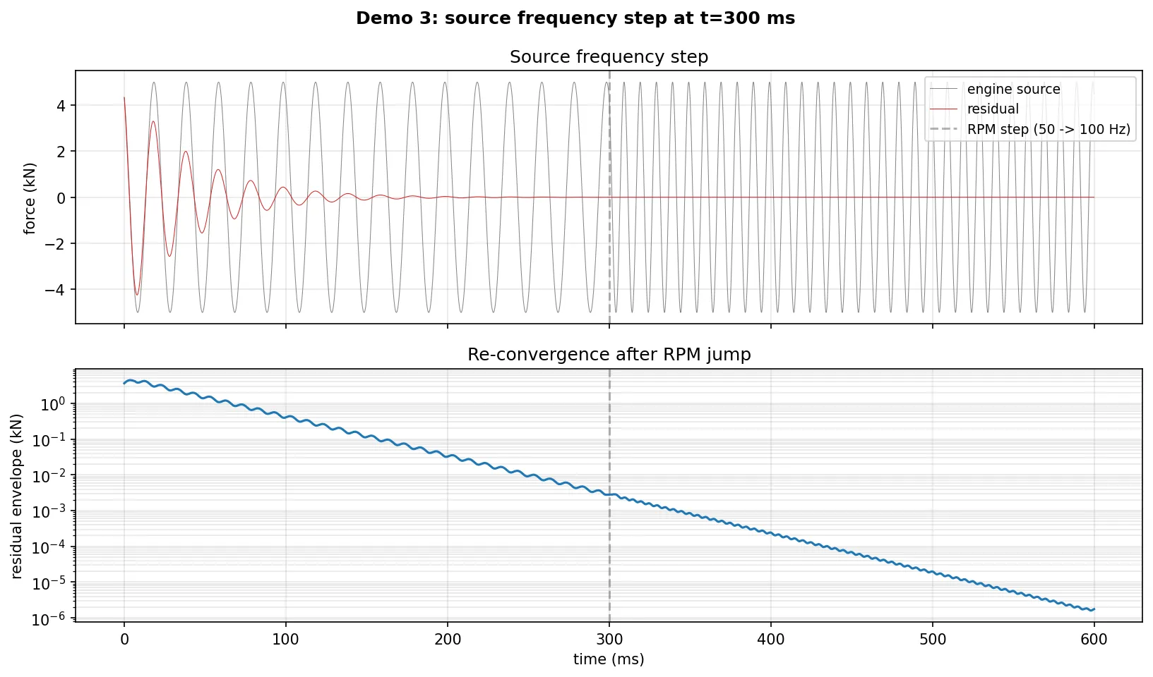
The phasor structure of the controller is frequency-invariant — weights have no time-dependence, so changing $\omega$ doesn’t reset them. But the optimal weights at the new $\omega$ are the same as at the old $\omega$ (assuming the source amplitude and phase are unchanged). So the controller converges at the new operating point in a fraction of $\tau$ , often before the engine even fully completes the RPM transition.

Real production active dampers track RPM continuously; this demo shows the simplest case (a discrete jump) to illustrate that the algorithm doesn’t break.

6. Demo 4 — actuator delay drives naive LMS unstable

Real actuators have lag: solenoid magnetic-field rise time, motor electrical time constant, drive-amplifier latency, A/D and D/A conversion. This adds a delay $D$ between the controller’s commanded force and the force that physically appears.

Naive LMS (which uses the current reference signal in its update law, not a delay-compensated one) becomes unstable when $D$ is large enough that the gradient direction rotates by more than 90° per update.

Approximately:

$D \cdot \omega \cdot \Delta t < \frac{\pi}{2} \quad \Rightarrow \quad D_\text{critical} \approx \frac{\pi}{2 \cdot \omega \cdot \Delta t}\ \text{samples}$

For $\omega = 628\ \text{rad/s}$ (= 100 Hz) and $\Delta t = 10^{-4}\ \text{s}$ : $D_\text{critical} \approx 25\ \text{samples} = 2.5\ \text{ms}$ .

Sweeping three delay values:

Actuator delay instability

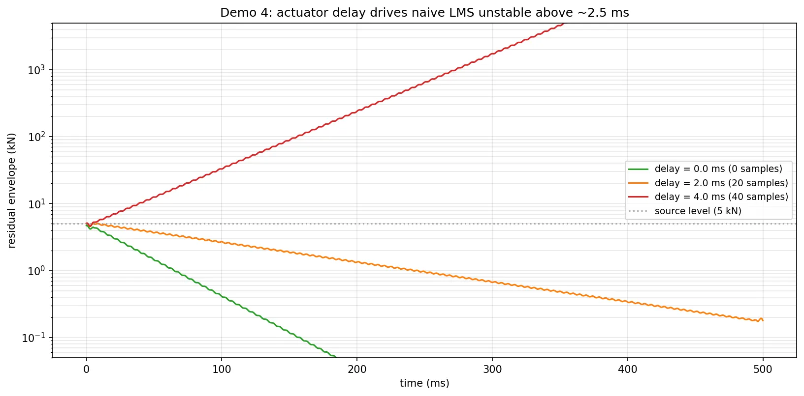
Delay	Final residual envelope	Status
0.0 ms	0 N	stable, full cancellation
2.0 ms	207 N	stable but with bounded leakage
4.0 ms	$5.6 \times 10^7$ N	UNSTABLE — residual blows up

The 4 ms case is the kind of failure mode that trashes hardware: the controller’s “cancellation” force grows exponentially because its sign relative to the actual residual has flipped. Real systems either stay below $D_\text{critical}$ (use fast actuators with ≤ 1 ms total latency), or use a smarter controller — Filtered-X LMS — that knows about the delay and pre-rotates the gradient to compensate. The latter is a one-line modification:

$\text{reference filter:} \quad c_\text{filtered}(t) = c(t - D\cdot\Delta t)$

$\text{update law:} \quad w_c \mathrel{-}= \mu \cdot e(t) \cdot c_\text{filtered}(t)$

FX-LMS extends the stable delay range from $\approx \pi/(2\omega)$ to many multiples of one period, making it the standard choice for production active-noise systems.

7. Where this lives in production hardware

Active mass damping at the source is one of three places to close the cancellation loop, mirroring the three layers of the source- to-chassis path from earlier chapters:

Layer	What’s cancelled	Where the actuator lives	Example
Source-side (this chapter)	engine block force	inside the engine accessories	active counter-rotating shaft, e.g. Mitsubishi pioneered this
Mount-side	mount-spring force	inside the engine mount	active mounts on Mercedes / Lexus V8s in the 2000s
Cabin-side	cabin acoustic pressure	speakers in the cabin	Bose / Lexus / Acura active noise cancellation

All three use the same LMS-style algorithm, just with different sensor and actuator placements. Production high-end vehicles typically stack all three: passive balance shafts cancel the known-magnitude inertial 2× (for free, mechanically), active mass damping at the source mops up the load-dependent residual, and cabin-side ANC trims whatever made it through.

The framework presented here covers all three with the same machinery — pick which signal is $e(t)$ and which actuator contributes $F_\text{act}(t)$ , the LMS update law is the same.

8. FAQ

Q1. The script implements LMS with no actuator-delay compensation. Why is it called “active mass damping” instead of “active force injection”?

Same idea, different historical naming convention. “Mass damping” descends from the original passive tuned-mass damper: a free mass on a spring attached to the structure, sized so its resonance absorbs energy at the structure’s problem frequency (the Stockbridge dampers on power lines, the 660-tonne ball at the top of Taipei 101). “Active mass damping” is the same idea with a controlled actuator force on the auxiliary mass instead of relying on a passive spring’s resonance. In active-noise-control terminology it would just be called “feedforward narrowband cancellation”. The algorithm is the same.

Q2. What sets the step size $\mu$ ?

A trade between convergence speed and steady-state misadjustment:

Too small $\mu$ : convergence is slow ( $\tau = 2/\mu$ samples). At $\mu = 1\times10^{-4}$ the controller takes ~2 seconds to converge — slow enough that a driver feels each throttle transition as a brief buzz before the controller catches up.
Too large $\mu$ : the controller overshoots and either oscillates around the optimum or, in extremis, diverges. The hard upper limit is $\mu < 2 / \lambda_\text{max}(R_{xx}) \approx 2$ for the unit-amplitude cosine-sine reference; in practice you stay well below to keep steady-state misadjustment low.

Production controllers use variable step size: large $\mu$ during transients (fast convergence), small $\mu$ once locked (low residual). Implementations include normalised LMS (NLMS), where $\mu_\text{eff} = \mu / E[\text{reference}^2]$ , and leaky LMS, which biases weights back toward zero to prevent drift.

Q3. Can the controller cancel multiple harmonics at once?

Yes — independently. Each harmonic $n$ gets its own weight pair $(w_{c,n}, w_{s,n})$ and its own LMS update using $\cos(n\cdot\omega\cdot t)$ and $\sin(n\cdot\omega\cdot t)$ as references. The actuator output is the sum across all harmonics:

$F_\text{act}(t) = \sum_n \left[ w_{c,n} \cdot \cos(n\cdot\omega\cdot t) + w_{s,n} \cdot \sin(n\cdot\omega\cdot t) \right]$

LMS updates for different harmonics are decoupled because the references are orthogonal (different frequencies have zero time- average product). Cancelling 1× crank, 2× crank, and firing frequency simultaneously is just three independent pairs of weights running in parallel — same algorithm three times.

Q4. What is “Filtered-X LMS” exactly?

The standard fix for actuator-delay or actuator-dynamics issues. The naive LMS update law assumes the actuator is instantaneous — that the force the controller commands is the force that arrives. When that’s wrong, the gradient direction is misaligned and the update step can overshoot or even point uphill.

Filtered-X LMS pre-filters the reference signal through an identified model $\hat{S}(z)$ of the actuator-plus-secondary-path dynamics, so the controller’s update uses what the actuator will deliver, not what it was commanded to deliver:

$c_\text{filtered}(t) = \hat{S}(z)\cdot c(t)$

$s_\text{filtered}(t) = \hat{S}(z)\cdot s(t)$

$w_c(t+\Delta t) = w_c(t) - \mu\cdot e(t)\cdot c_\text{filtered}(t)$

$w_s(t+\Delta t) = w_s(t) - \mu\cdot e(t)\cdot s_\text{filtered}(t)$

$\hat{S}(z)$ is identified once at design time by injecting a known signal through the actuator and measuring the response. As long as the real plant doesn’t drift far from the model, FXLMS extends the stable delay range from $\approx \pi/(2\omega)$ (Demo 4’s wall) to several multiples of the cancellation period.

Q5. How does this interact with the engine mount transmissibility?

Cleanly. Active source-side damping reduces the engine-side phasor before it reaches the mount. So the mount sees a reduced source, and its already-good high-frequency isolation amplifies the benefit: if active damping cuts the source by 99 % and the mount isolates by 99 %, total chassis-side reduction is 99.99 %.

Concretely with the engine-mount chapter’s worked example:

Source: 7400 N at 100 Hz
After active damping: residual $\approx$ 0.5 N (99.99 % cancellation)
After soft-mount transmission (T = 0.0064): chassis force $\approx$ 3 mN

That is sub-perceptual. Production hybrid powertrains achieve this kind of stack to deliver “I4 cabin smoothness on V12 mounts” — the small engine vibrates, but you cannot feel it.

Q6. What can break this loop in the real world?

The usual control-systems gotchas:

Sensor noise raises the steady-state residual floor. The controller can’t cancel below the measurement noise level.
Reference noise (a noisy crank-angle sensor) corrupts the cosine/sine references, biasing convergence. Production systems use phase-locked loops on the crank trigger to clean this up.
Plant drift (the secondary path $\hat{S}(z)$ changing with temperature, aging) causes FXLMS to mis-align gradually. Adaptive plant identification (“on-line modelling”) fixes it.
Limit cycles can appear if the actuator saturates. The controller commands force outside the actuator’s range; the saturated output is no longer a clean phasor; LMS can lock onto the harmonic distortion and oscillate. Production systems use saturation-aware variants like leaky LMS.
Multiple sensor / actuator paths can interact. With more than one cancellation point, the cross-coupling between the secondary paths needs explicit identification (Multiple-Reference Multiple- Output FXLMS).

None of these break the framework; they just demand the next control-systems extension. The narrowband LMS in this chapter is the simplest member of a family that scales up to all of them.

9. What’s next

The active-damping framework opens out further along two axes:

Multi-channel active control — multiple sensors and multiple actuators distributed around the engine and chassis. Cancellation is no longer a single phasor pair but a matrix of phasors that must be coordinated. The “MIMO FXLMS” generalisation handles it with the same gradient-descent core; the bookkeeping just grows.
Model-predictive control (MPC) — explicitly optimise weights over a future time horizon given a model of the plant. More computationally demanding than LMS but handles constraints (actuator saturation, bandwidth limits) and lookahead (predicting RPM trajectory from throttle input) more cleanly.
Combined source / mount / cabin layers — not a new algorithm, but a coordinated deployment. Each layer cancels what the next layer can’t — production high-end vehicles stack all three and hand a sub-perceptual residual to the driver.

This chapter closes the analytical loop on the multi-cylinder series: from single-cylinder simulation, through phasor sums for multi-cylinder layouts, through V-engines and combustion, through balance shafts and engine mounts, to closed-loop active control. Every chapter has used the same framework; each new feature adds one term to the same EOM or the same phasor sum.

Files and scripts referenced

active_mass_damping.py — this chapter’s script. ActiveDamper class implementing narrowband LMS with optional actuator-delay buffer, simulate() driver, four demo_* functions producing the PNGs above.
No additions to _common.py; the LMS update is local to the damper class.
Connects directly to the Balance Shafts chapter (open-loop version of the same idea) and the Engine Mounts chapter (where the residual after this chapter’s cancellation feeds the mount transmissibility).